import json
import pathlib
from os import environ
from typing import Generator, NamedTuple, TypedDict

from matplotlib.axes import Axes
import seaborn as sns
import pandas as pd
import numpy as np
import matplotlib.pyplot as plt

from matplotlib.animation import FuncAnimation


# NOTE: Constants. These will determine how long it will take for this document
#       to render. Further, changing these documents can result in an error
#       from deno with the message ``ERROR: RangeError: Maximum call stack size
#       exceeded``.
LOGISTIC_X0_DEFAULT = float(environ.get("LOGISTIC_X0_DEFAULT", "0.9"))
LOGISTIC_STEP_SIZE = float(environ.get("LOGISTIC_STEP_SIZE", "0.01"))
LOGISTIC_STEP_SIZE_RR = float(environ.get("LOGISTIC_STEP_SIZE_RR", "0.02"))
LOGISTIC_ITERATIONS = int(environ.get("LOGISTIC_ITERATIONS", "1000 "))
LOGISTIC_ITERATIONS_KEPT = int(environ.get("LOGISTIC_ITERATIONS_KEPT", "100"))

DIR = pathlib.Path(".").resolve()
LOGISTIC_DATA_BIFURCATION = (
    DIR / f"logistic-bifurcation-{LOGISTIC_ITERATIONS}-{LOGISTIC_STEP_SIZE}.csv"
)
LOGISTIC_DATA_COBWEB_RR = (
    DIR / f"cobweb-{LOGISTIC_STEP_SIZE}-{LOGISTIC_STEP_SIZE_RR}.json"
)


def logistic_point(
    rr: float,
    xx: float,
    *,
    power: int = 1,
    _power: int = 0,
) -> float:
    """Compute the value of the logistic map for some coefficient `rr` and
    number `xx`.
    """

    _power += 1

    xx_next = rr * xx * (1 - xx)
    if _power == power:
        return xx_next

    return logistic_point(rr, xx_next, power=power, _power=_power)


def _logistic_array(rr: float, xx, *, power=1):
    """Helper for ``logistic_array``."""

    # NOTE: Numpy multiplies elements stepwise.
    yy, _power = xx, 0
    while _power < power:
        yy = rr * yy * (1 - yy)
        _power = _power + 1

    return yy


def logistic_array(
    rr: float,
    *,
    step: float = 0.001,
    power: int = 1,
):
    """Compute the graph of the logistic map on the closed interval $[0, 1]$."""

    xx = np.arange(0, 1 + step, step=step)
    yy = _logistic_array(rr, xx, power=power)

    return pd.DataFrame(dict(xx=xx, yy=yy))


def logistic_point_sequence(
    rr: float,
    xx: float,
    *,
    iterations: int = LOGISTIC_ITERATIONS,
) -> Generator[float, None, None]:
    """Iterate the logistic sequence starting at `xx` for coefficient `rr` for
    `iterations` number of steps."""

    if not (0 <= xx <= 1):
      raise ValueError("`xx` must be between `0` and `1`.")

    yield xx

    iteration = 0
    while (iteration := iteration + 1) < iterations:
yield (xx := logistic_point(rr, xx))The Logistic Map and Chaos
python
math
The logistic map: Animations and properties.
Keywords
logistic map, logistic, map, chaos, python, seaborn, numpy, diagram, cobweb, bifurcation, polynomial
This was my first quarto blog post that I wrote! Now I have added much more content than there was before.
The logistic map was used to explain chaos occurring in simple situations in a physics class I took back in college. This class went far deeper into the subject matter than this blog post does at the moment, but I might come back and write more in this blog post later.
For now, this will demonstrate some of the basic properties of the recurrence relation, provide some definitions, and showcase some cool animations.
The Logistic Map and Recurrence Relations
The logistic map is a function defined as
\[\begin{equation} l_r: x \mapsto rx(1-x) \end{equation}\]
where \(r \in [0, 4]\) and \(x \in [0, 1]\). A logistic sequence is defined as
\[\begin{equation} \lambda_r = \{l_r^k(x_0): k \in N\} \end{equation}\]
for some \(x_0\) and \(r\) and is defined by the recurrence relation
\[\begin{equation} x_{k+1} = rx_k(1-x_k) \end{equation}\]
In this case, the exponent on \(\lambda_r\) is the degree of composition; more precisely, \(\lambda^3_r(x) = \lambda_r(\lambda_r(\lambda_r(x)))\) for instance.
It is easy to write out some python functions that will compute the values of the logistic sequence:
Visualizing Sequences - The Cobweb Daiagram
An interseting question is how to plot the logistic sequence. This can be done by plotting the points on a line - which is pretty boring and does not show the relationship between the points.
A cobweb diagram can be used to visualize the convergence (or lack there of) of a logistic sequence and the relationship between the points. The procedure for creating the diagram is as follows:
- An initial input \(x_0\) is chosen. This can be written as the point \((x_0, x_0)\) on the graph.
- The output \(x_1 = \lambda_r(x_0)\) is computed. This can be represented as the point \((x_0, x_1)\).
- The next point will be \((x_1, x_1)\), directly on the line \(x = y\).
- Since the next input into the logistic map is \(x_1\), we follow the \(x\) projection onto the logistic maps graph to get \((x_1, x_2 := lambda(x_1))\). This step is just step \(2\).
- Next step three is repeated for \(x_2\).
In the most explicit form this is
\[\begin{multline} \{ \\ (x_0, x_0), \\ (x_0, \lambda_r(x_0)), (\lambda_r(x_0), \lambda(x_0)), \\ (\lambda(x_0), \lambda^2(x_0)), (\lambda^2(x_0), \lambda^2(x_0))), \\ (\lambda^2(x_0), \lambda^3(x_0)), (\lambda^3(x_0), \lambda^3(x_0)), \\ ... \\ (\lambda^{k-1}(x_0), \lambda^{k}(x_0)), (\lambda^k(x_0), \lambda^k(x_0)), \\ ... \\ \} \end{multline}\]
Moreover, if \(l_r = \{a_k := \lambda^k_r(x_0), k \in N\}\) is a logistic sequence, then we are just plotting
\[\begin{equation} \{ (a_0, a_0), (a_0, a_1), (a_1, a_1), (a_1, a_2), (a_2, a_2), ..., (a_k, a_{k+1}), (a_{k+1}, a_{k+1}), ... \} \end{equation}\]
If \(\lambda_r\) is plotted along with \(x \mapsto x\), the elements of the cobweb sequence should lie on either line, alternating between them. The sequence of points above can be computed and visualized using the script in Figure 1.
Point = tuple[float, float]

class Line(NamedTuple):
  xx: Point
  yy: Point

class CobwebCalculator:
  def __init__(
      self,
      iterations: int = 100,
             ):

    self.iterations = iterations

  def iter_cobweb( self, rr: float, x0: float ) -> Generator[Point, None, None]:
      """Iterates the elements of the cobweb sequence."""
      iteration, xx = 0.0, x0
      while (iteration := iteration + 1) < self.iterations:
          yield (xx, xx)
          yield (xx, xx := logistic_point(rr, xx))


  def iter_cobweb_segments( self, rr: float, x0: float) -> Generator[Line, None, None]:
      """Iterates tuples representing the line segments making up the cobweb
      diagram"""

      points = self.iter_cobweb(rr, x0)
      xx, yy = zip(*points)
      for xx_coords, yy_coords in zip(zip(xx[:-1], xx[1:]), zip(yy[:-1], yy[1:])):
          yield Line(xx_coords, yy_coords)

  def daiagram_cobweb(
      self,
      rr: float,
      x0: float = LOGISTIC_X0_DEFAULT,
      *,
      output: pathlib.Path | None = None,
      interval: int = 50,
  ) -> None:
      """Creates the cobweb diagram animation segments for a fixed value of
      `rr` and `x0`."""

      output = output if output is not None else DIR / f"cobweb-{rr}-{x0}.gif"
      if output.exists():
        return

      # Do not fear, this just uses the values from the scope below when called.
      def update_cobweb(frame: int):
          data_line = data_cobweb[frame]
          return ax.plot(data_line.xx, data_line.yy, color="red")

      data_logistic = logistic_array(rr)
      data_cobweb = list(self.iter_cobweb_segments(rr, x0))
      frames = self.iterations

      ax: Axes
      fig, ax = plt.subplots()
      ax.set_ylim(0, 1)
      ax.set_xlim(0, 1)
      ax.set_title(f"Cobweb Daiagram for `x0={x0}` and `rr={rr}`")

      # Plot the logistic map and the identity.
      ax.plot(xx := data_logistic["xx"], data_logistic["yy"], color="blue")
      ax.plot(xx, xx, color="green")

      # Animate cobweb.
      animation = FuncAnimation(fig, update_cobweb, frames=frames, interval=interval)
      if output is not None:
animation.save(output, writer="pillow")matplotlib. See the output in Figure 2.
The code code in Figure 1 can be used as follows:
# Sequences that converge rapidly (quadratic convergence)
cobweb_calculator = CobwebCalculator(iterations=20)
cobweb_calculator.daiagram_cobweb(2, 0.9)
cobweb_calculator.daiagram_cobweb(1, 0.7)

# Sequences that do not converge
cobweb_calculator = CobwebCalculator()
cobweb_calculator.daiagram_cobweb(3, 0.2)
cobweb_calculator.daiagram_cobweb(3.2, 0.4)
cobweb_calculator.daiagram_cobweb(3.8, 0.9)
cobweb_calculator.daiagram_cobweb(3.5, 0.5)
plt.close()

The code in Figure 3 will plot cobwebs varied smoothly over \(r\) on the interval \([0, 4]\). This will show how convergence varies as the value of \(r\) varies.
def load_cobweb_rr(x0, path: pathlib.Path):
    """Load the data if it exists already instead of generating it."""

    if path.exists():
        with open(path, "r") as file:
            raw = json.load(file)

        return {float(rr): df_raw for rr, df_raw in raw["data_cobweb"].items()}, {
            float(rr): pd.DataFrame(json.loads(df_raw))
            for rr, df_raw in raw["data_logistic"].items()
        }

    calculator = CobwebCalculator()
    rrs = np.arange(0, 4, LOGISTIC_STEP_SIZE_RR)
    data_cobweb = {
        rr: list(zip(*calculator.iter_cobweb(rr, x0))) for rr in rrs
    }
    data_logistic = {rr: logistic_array(rr) for rr in rrs}

    with open(LOGISTIC_DATA_COBWEB_RR, "w") as file:
        json.dump(
            {
                "data_cobweb": data_cobweb,
                "data_logistic": {rr: df.to_json() for rr, df in data_logistic.items()},
            },
            file,
        )

    return (data_cobweb, data_logistic)


def diagram_cobweb_rr(path: pathlib.Path,interval: int = 200 ):
    """Create the cobweb diagram animation for a fixed starting point and a
    varied $r$."""

    x0 = LOGISTIC_X0_DEFAULT
    data_cobweb, data_logistic = load_cobweb_rr(x0, path)

    fig, ax = plt.subplots()

    rrs = np.array(sorted(data_cobweb))
    rr0 = min(rrs)

    (line_cobweb,) = ax.plot(
        data_cobweb[rr0][0],
        data_cobweb[rr0][1],
        color="blue",
    )
    (line_logistic,) = ax.plot(
        data_logistic[rr0]["xx"],
        data_logistic[rr0]["yy"],
        color="red",
    )
    ax.plot(xx := data_logistic[rr0]["xx"], xx, color="green")
    tx = ax.text(0, 1.1, f"r = {rr0}")

    def update_cobweb_rr(frame_rr):
        line_cobweb.set_xdata(data_cobweb[frame_rr][0])
        line_cobweb.set_ydata(data_cobweb[frame_rr][1])

        line_logistic.set_xdata(data_logistic[frame_rr]["xx"])
        line_logistic.set_ydata(data_logistic[frame_rr]["yy"])

        tx.set_text(f"r = {round(frame_rr, 2)}")

        return (line_cobweb, line_logistic)

    frames = list(rrs)
    frames += frames[-1: 0]
    animation = FuncAnimation( fig, update_cobweb_rr, frames=frames, interval=interval)
    plt.close()
    return animation

if not (_ := DIR / "cobweb-rr-0.9.gif").exists():
    animation = diagram_cobweb_rr(interval=100, path=_)
    animation.save(_, writer="pillow")
Attractors
Often there will be not a single attractor, but many. For instance, the sequence \(\{\lambda^k_r(x_0)\}\) between the values of \(3\) and \(3.4\) will be the union of two convergent subsequences. For now, we can use the rough rule that for may points falling within a small epsilon we probably have a convergent subsequence.
class AttractorCalculator:
  def __init__(self,
      epsilon: float = 0.0001,
      iterations: int = LOGISTIC_ITERATIONS,
      iterations_kept: int=LOGISTIC_ITERATIONS_KEPT,
               ):

    self.epsilon = epsilon
    self.iterations = iterations
    self.iterations_kept = iterations_kept

  def get_set(
    self,
      rr: float,
      xx: float,
  ) -> set[int]:
      """
      Assumes that points `epsilon` close will make a convergent subsequence.

      Not the most rigorous, but good enough to show loci of the sequence.
      """

      attractors = set()

      index_min = self.iterations - self.iterations_kept
      seq = logistic_point_sequence(rr,xx, iterations=self.iterations)
      candidates = (pt for index, pt in enumerate(seq) if index > index_min)

      for elem in candidates:

        # NOTE: If no attractors, add the element.
        if not attractors:
            attractors.add(elem)
            continue

        # NOTE: If some points are close, replace them with this point.
        close = set(attr for attr in attractors if abs(elem - attr) < self.epsilon )
        if close:
          attractors -= close
          attractors.add(elem)
        else:
          attractors.add(elem)

      return attractors

  def generate_points(self, rr: float, xx:float) -> Generator[tuple[float, float, float], None, None]:
      attractors = self.get_set(rr, xx)
yield from ((rr, xx, attr) for attr in attractors)import rich
import rich.console
import io
def attractors_print(
rr: float,
xx: float,
# *,
# console: Console
note: str | None = None,
)-> None:
attractors = attractor_calculator.get_set(rr, xx)
console.rule(title=f"Attractors for `{rr=}` and `{xx=}`.")
if note is not None:
console.print(note)
console.print()
console.print(attractors)
console = rich.console.Console(record=True, width=100, file=io.StringIO())
attractor_calculator = AttractorCalculator()
attractors_print(0, 1, note="[yellow]When `rr` is `0`, the sequence should only output `0`.")
attractors_print(2, 0.5, note="[yellow]When `rr` is `2` and `x=0.5`, the sequence is only ever `2 * 0.5 * (1 - 0.5) = 0.5`.")
attractors_print(3.2, 0.1, note="[yellow]Should have two attractors.")
attractors_print(3.5, 0.8, note="[yellow]Should have four attractors.")
console.save_svg("attractors-algo-outputs.svg")
Bifurcation Diagram
In this section, we will create a bifurcation diagram for the logistic map. This bifurcation diagram is used to show the attractors for the logistic sequence depending on \(r\).
Since logistic_attractors can generate attractors for the logistic sequence at a point with reasonable accuracy, it is relatively easy to generate a dataframe that will contain points for the logistic sequence. This is done in Figure 7. It accepts a number of chunks so that ranges for different values of \(r\) can be plotted differently (in different resolutions or with a different number of starting points).
import numpy.typing as npt
FloatArray = npt.NDArray[np.float64]


class BifurcationChunkConfig(TypedDict):
  rrs: FloatArray
  xxs: FloatArray


class BifurcationCalculator:
  """
  Computes the attractors over the whole domain and put into a dataframe.
  Save the dataframe to save on overhead.

  Since different regions require different resolutions and a different number
  of starting points, `chunks` should be used to set render settings for each
  piece of the domain.
  """

  attractor_calculator: AttractorCalculator

  def __init__(self,
               chunks: list[BifurcationChunkConfig], *,
               file_name: str,
               attractor_calculator: AttractorCalculator | None = None,
               data: pd.DataFrame | None = None,
               ):

    self.file_path =   DIR / file_name
    self.chunks = chunks
    self.attractor_calculator = attractor_calculator or AttractorCalculator()

    data_from_file = False
    if self.file_path.exists() and not data:
      data_from_file = True
      data = pd.read_csv(self.file_path)

    self.data = data if data is not None else self.create_data()
    self.data_from_file = data_from_file

  def save(self):
    if self.data_from_file:
      return

    self.data.to_csv(self.file_path)

  def create_data_chunk(
    self, config: BifurcationChunkConfig,
  ) -> pd.DataFrame:
      point_data = (
        ( index, *attractor )
        for rr in config["rrs"]
        for index, x_0 in enumerate(config["xxs"])
        for attractor in self.attractor_calculator.generate_points(rr, x_0)
      )
      return pd.DataFrame(data=point_data, columns=["iteration_number", "rr", "x0", "attractor"])


  def create_data(self) -> pd.DataFrame:
    chunks = (self.create_data_chunk(chunk) for chunk in self.chunks)
return pd.concat(chunks)CSV files.
The Bifurcation Diagram
With the code from Figure 7 we can generate a plot of the bifurcation diagram with regions in different resolutions. As the graph becomes more chaotic, more features can be noticed by increasing the sample size in \(r\) in each region and starting sequences for different values of \(x_0\) makes more sense since there will be a greater number of attractors.
calc = BifurcationCalculator(
chunks=[
{
"rrs": np.linspace(0, 3, 750),
"xxs": np.linspace(0, 1, 3),
},
{
"rrs": np.linspace(3, 3.4, 150),
"xxs": np.linspace(0, 1, 5),
},
{
"rrs": np.linspace(3.4, 3.6, 300),
"xxs": np.linspace(0, 1, 25),
},
{
"rrs": np.linspace(3.6, 4, 1200),
"xxs": np.linspace(0, 1, 25)
}
],
file_name="simple.csv",
)
calc.save()
regions = dict(
zero =calc.data.query("0 <= rr < 1"),
single = calc.data.query("1 <= rr < 3 and attractor > 0"),
double= calc.data.query("3 <= rr < 3.4 and attractor > 0"),
cascade = calc.data.query("3.4 <= rr < 3.6 and attractor > 0"),
chaos = calc.data.query("3.6 <= rr <= 4 and attractor > 0")
)
def create_bifurcation_full():
"""
Generate the full plot. Notice that the query for an attractor greater than
zero does not require rounding.
"""
ax_full = regions["zero"].plot.scatter(x="rr", y="attractor", s=0.1, c="blue")
regions["single"].plot.scatter(x="rr", y="attractor", s=0.1, c="blue", ax=ax_full)
regions["double"].plot.scatter(x="rr", y="attractor", s=0.01, c="purple", ax=ax_full)
regions["cascade"].plot.scatter(x="rr", y="attractor", s=0.0001, c="red", ax=ax_full)
regions["chaos"].plot.scatter(x="rr", y="attractor", s=0.00001, c="orange", ax=ax_full)
ax_full.set_title("Logistic Map Bifurcation Daiagram - Full")
ax_full.figure.savefig("./bifurcation-full.png")
plt.close()
def create_bifurcation_cascade():
"""Generate the doubling cascade region."""
ax_cascade = regions["cascade"].plot.scatter(x="rr", y="attractor", s=0.00001, c="orange")
regions["chaos"].plot.scatter(x="rr", y="attractor", s=0.00001, ax=ax_cascade, c="red")
ax_cascade.set_title("Logistic Map Bifurcation Daiagram - Cascade")
ax_cascade.figure.savefig("./bifurcation-casade.png")
plt.close()
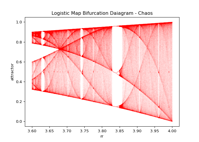
def create_bifurcation_chaos():
"""Plot the chaotic region."""
ax_chaos = regions["chaos"].plot.scatter(x="rr", y="attractor", s=0.00001, c="red")
ax_chaos.set_title("Logistic Map Bifurcation Daiagram - Chaos")
ax_chaos.figure.savefig("./bifurcation-chaos.png")
plt.close()
create_bifurcation_full()
create_bifurcation_cascade()
create_bifurcation_chaos()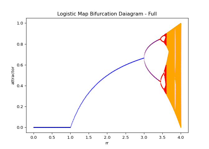
create_bifurcation_full. For descriptions of the color coating, see ?@tbl-bifurcation-keys.
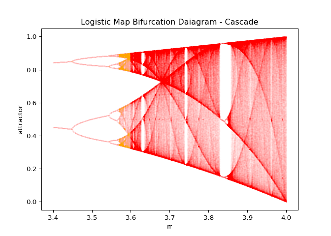
create_bifurcation_cascade.
| Region | Color | Logistic Sequence Behavior | Number of Samples in \(r\) | Number of samples in \(x\) |
|---|---|---|---|---|
| $0 r | Blue | Converges to zero or a single point. | 750 | 3 |
| $3 r | Purple | Initial doubling. | 150 | 5 |
| $3.4 r | Red | Second doubling and cascade. | 300 | 25 |
| $3.6 | Orange | Chaotic | 1200 | 25 |
A few well known facts about the logistic map are apparent from the bifurcation diagrams shown in Figure 8:
- Below a value of three, the logistic sequence actually converges
- For \(r\) between \(3\) and roughly \(3.4\), the logistic map will have two distinct convergent subsequences.
- For values of roughly \(r=3.4\) up until roughly \(3.6\) there will be four distinct convergent subsequences.
- The bifurcation cascade blows up after approximately \(r=3.6\).
These facts can be proven by solving the recurrence relation but are beyond the scope of this article.
Distribution of Attractors
def create_attractor_distribution():
  data = calc.data.query("rr > 3.55 and attractor > 0")[["rr", "attractor"]]
  data["attractor"] = data["attractor"].round(4)

  ax = sns.histplot(data["rr"], bins=100)
  ax.set_title("Distribution of Attractors In Cascade Region")
  ax.figure.savefig("attractor-distribution-cascade.svg")
  plt.close()

  return data

attractor_dist = create_attractor_distribution()
Subsets of the Bifurcation Diagram
In Figure 8 (c), there is a region where the number of attractors becomes dramatically less. Using BifurcationCalculator we can generate the high quality image of this region in Figure 10.
calc_self_similar = BifurcationCalculator([
  {
    "rrs": np.linspace(3.83, 3.856, 1000),
    "xxs": np.linspace(0.4, 0.6, 25),
  }
], file_name="./self-similar.csv")
calc_self_similar.save()

ax_self_similar = calc_self_similar.data.query("0.4 < attractor < 0.6").plot.scatter(x="rr", y="attractor", s=0.0001)
ax_self_similar.figure.savefig("./bifurcation-self-similar.png")
plt.close()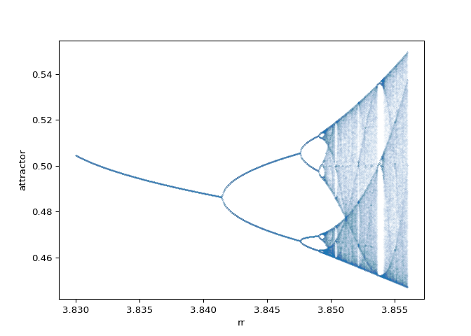
Logistic Compositions
In this context, logistic compositions refers to the sequence of functions
\[\begin{equation} \{\lambda_r^k: k \in N\} \end{equation}\]
for some \(r\). This sequence exists in the space of continuously differentiable functions on the closed unit interval, which is notated as \(C^\infty([0, 1])\). Here I will not bother to proof that polynomials are continuously differentiable as this is easy to find in any analysis book or online. In fact the only point of mentioning that this sequence exists in this space (in this current version of the blog post) is drive home that this is a sequence of functions, not numbers.
It is possible to make some nice graphs of the logistic function and its composition with itself. The following code is used to generate the subsequent diagrams:
def diagram_composition(rr: float, frames: int):
    """Create the composition animation for some ``rr``."""

    def update_composition(frame):
        line.set_ydata(data_composition[frame]["yy"])

        tx.set_text(f"k = {frame}")
        return (line,)

    data_composition = [logistic_array(rr, power=k + 1) for k in range(frames)]
    fig, ax = plt.subplots()

    tx = ax.text(0, 1.1, "k = 0")
    (line,) = ax.plot(
        xx := data_composition[0]["xx"],
        data_composition[0]["yy"],
        color="blue",
    )
    ax.plot(xx, xx, color="red")
    animation = FuncAnimation(fig, update_composition, frames=frames)

    plt.close()
    return animation
The plot below shows \(\lambda_4^k\) (the compositions):
animation = diagram_composition(4, frames=64)
if not (output_path := DIR / "composition-4.gif").exists():
    animation.save(output_path, writer="pillow")
Seeing the evolutions of the above plot it is clear why the logistic sequence does not converge for higher values of \(r\). In the case that \(r = 3\) the sequence does converge (as we will see in the next section) and the compositions have maxima and minima that are in a smaller range.
animation = diagram_composition(3, frames=9)
if not (output_path := DIR / "composition-3.gif").exists():
    animation.save(output_path, writer="pillow")
Finally, when \(r=2\) the compositions appears to only have \(3\) extrema no matter the degree of composition:
animation = diagram_composition(1, frames=11)
if not (output_path := DIR / "composition-1.gif").exists():
    animation.save(output_path, writer="pillow")